지금까지 우리는 시계열 데이터의 구성 요소를 이해하고, 다양한 예측 모델들의 특징과 활용법을 살펴보았습니다. 이제 이러한 지식을 실전에 적용하는 마지막 단계로, 가장 중요한 “지속 가능한 운영”에 대해 알아보겠습니다.
이전 글 보기: 데이터로 보는 트렌드: 시계열 데이터의 비밀(1)
데이터로 보는 트렌드: 시계열 데이터의 비밀(2)
Part 3: 실전 활용과 모니터링
시계열 예측 모델을 실전에 적용할 때 가장 중요한 것은 지속 가능성입니다. 아무리 정교한 모델이라도 시간이 지남에 따라 예측 정확도가 감소할 수 있으며, 이는 비즈니스 환경 변화, 소비자 행동 패턴 변화, 시장 구조의 변동 등 다양한 요인에 기인합니다. 따라서 프로덕션 환경에서는 모델의 성능을 지속적으로 모니터링하고, 적절한 시점에 모델을 재학습하거나 교체하는 체계적인 프로세스가 필수적입니다.
모니터링 및 재학습 프로세스

모델 성능 모니터링
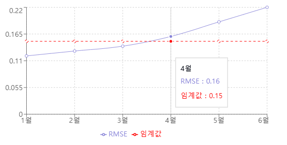
성능 모니터링은 RMSE, MAE, MAPE 등 주요 평가 지표를 기반으로 진행됩니다. 이러한 지표들의 변화를 추적하면서 잔차 분석을 통해 예측의 편향성을 검토합니다. 또한 신뢰구간의 정확도를 지속적으로 확인하고, 이상치를 탐지하여 적절히 처리합니다. 이러한 지표들의 시간에 따른 추이를 시각화하여 주기적으로 분석하면, 모델 성능의 변화를 직관적으로 파악할 수 있습니다.
드리프트 감지 및 대응
시간이 지남에 따라 발생하는 성능 저하는 크게 두 가지 관점에서 모니터링합니다.
- 데이터 드리프트: 입력 데이터의 분포 변화 탐지
- 컨셉트 드리프트: 입력-출력 관계의 변화 포착
이러한 드리프트는 초기 설정한 베이스라인 성능과 현재 지표의 상대적 변화를 통해 판단하며, 지표 변화율이 특정 임계값을 초과할 경우 드리프트가 발생했다고 판단합니다. 시계열의 계절성과 추세 변화도 함께 관찰하며, 통계적 검정을 통해 변화의 유의성을 확인합니다.
효과적인 재학습 전략
모델 재학습을 위한 트리거 기준을 설정합니다. 고정 윈도우나 슬라이딩 윈도우 방식을 활용하여 재학습을 수행하며, 상황에 따라 점진적 학습 또는 전체 재학습 방식을 선택합니다. 모든 모델 버전은 체계적으로 관리되어 필요시 이전 버전으로의 롤백이 가능해야 합니다.
실시간 예측 시스템 운영
실제 운영 환경에서는 배치 처리와 실시간 예측이 모두 필요합니다. 이를 위해 특성 생성 파이프라인을 자동화하고, 예측 결과를 체계적으로 저장하고 관리합니다. 새로운 기능이나 모델은 A/B 테스트를 통해 검증한 후 적용합니다.
비즈니스 관점의 성과 분석
예측 모델의 성능은 단순한 정확도를 넘어 비즈니스 임팩트 관점에서 평가되어야 합니다. 예측 오차가 실제 비즈니스에 미치는 영향을 분석하고, 비용-효익 분석을 통해 모델 개선의 우선순위를 결정합니다. 또한 예측의 불확실성을 고려한 의사결정 체계를 구축하고, 이해관계자들에게 적절한 형태로 결과를 리포팅합니다.
import pandas as pd
import numpy as np
from typing import Dict, List, Optional, Tuple
from datetime import datetime, timedelta
import logging
from dataclasses import dataclass
import matplotlib.pyplot as plt
from scipy import stats
from pathlib import Path

@dataclass
class ModelMetrics:
    """시계열 예측 모델의 성능 지표를 저장하는 데이터 클래스"""
    mae: float
    rmse: float
    mape: float
    timestamp: datetime
    prediction_horizon: str  # 예: '1d', '1h', '15min'

    def to_dict(self) -> Dict:
        """메트릭을 딕셔너리 형태로 변환"""
        return {
            'mae': self.mae,
            'rmse': self.rmse,
            'mape': self.mape,
            'timestamp': self.timestamp,
            'prediction_horizon': self.prediction_horizon
        }

class TimeSeriesMonitor:
    """시계열 예측 모델 모니터링 시스템"""

    def __init__(
        self,
        model_name: str,
        metric_thresholds: Dict[str, float],
        monitoring_window: int = 30,
        logs_dir: Optional[str] = None
    ):
        """
        Args:
            model_name: 모니터링할 모델의 이름
            metric_thresholds: 각 메트릭별 임계값 (예: {'mae': 100, 'rmse': 150})
            monitoring_window: 모니터링 기록을 유지할 기간 (일)
            logs_dir: 로그 파일을 저장할 디렉토리 경로
        """
        self.model_name = model_name
        self.metric_thresholds = metric_thresholds
        self.monitoring_window = monitoring_window
        self.metrics_history: List[ModelMetrics] = []
        self.baseline_metrics: Optional[ModelMetrics] = None
        self.logger = self._setup_logger(logs_dir)

    def _setup_logger(self, logs_dir: Optional[str] = None) -> logging.Logger:
        """로깅 설정"""
        logger = logging.getLogger(f"tsmonitor_{self.model_name}")
        logger.setLevel(logging.INFO)

        # 파일 핸들러 설정
        if logs_dir:
            log_path = Path(logs_dir) / f"{self.model_name}_monitor.log"
            file_handler = logging.FileHandler(log_path)
            file_handler.setFormatter(
                logging.Formatter('%(asctime)s - %(name)s - %(levelname)s - %(message)s')
            )
            logger.addHandler(file_handler)

        # 콘솔 핸들러 설정
        console_handler = logging.StreamHandler()
        console_handler.setFormatter(
            logging.Formatter('%(name)s - %(levelname)s - %(message)s')
        )
        logger.addHandler(console_handler)

        return logger

    def calculate_metrics(
        self,
        y_true: np.ndarray,
        y_pred: np.ndarray,
        prediction_horizon: str = '1d'
    ) -> ModelMetrics:
        """성능 지표 계산"""
        if len(y_true) != len(y_pred):
            raise ValueError("실제값과 예측값의 길이가 일치하지 않습니다.")

        # 0으로 나누는 것을 방지
        y_true = np.where(y_true == 0, np.finfo(float).eps, y_true)

        mae = np.mean(np.abs(y_true - y_pred))
        rmse = np.sqrt(np.mean((y_true - y_pred) ** 2))
        mape = np.mean(np.abs((y_true - y_pred) / y_true)) * 100

        return ModelMetrics(
            mae=mae,
            rmse=rmse,
            mape=mape,
            timestamp=datetime.now(),
            prediction_horizon=prediction_horizon
        )

    def detect_drift(
        self,
        reference_data: np.ndarray,
        current_data: np.ndarray,
        threshold: float = 0.05
    ) -> Tuple[bool, float]:
        """분포 드리프트 감지"""
        statistic, p_value = stats.ks_2samp(reference_data, current_data)
        is_drift = p_value < threshold

        if is_drift:
            self.logger.warning(
                f"데이터 드리프트 감지! p-value: {p_value:.4f} (임계값: {threshold})"
            )

        return is_drift, p_value

    def update_metrics(self, new_metrics: ModelMetrics) -> None:
        """메트릭 업데이트 및 알림 확인"""
        self.metrics_history.append(new_metrics)

        # 모니터링 기간 관리
        cutoff_date = datetime.now() - timedelta(days=self.monitoring_window)
        self.metrics_history = [
            m for m in self.metrics_history
            if m.timestamp > cutoff_date
        ]

        # 베이스라인 설정 (첫 메트릭)
        if self.baseline_metrics is None:
            self.baseline_metrics = new_metrics
            self.logger.info("베이스라인 메트릭이 설정되었습니다.")

        self._check_alerts(new_metrics)
        self._check_trends()

    def _check_alerts(self, metrics: ModelMetrics) -> None:
        """임계값 초과 확인"""
        for metric_name, threshold in self.metric_thresholds.items():
            current_value = getattr(metrics, metric_name)
            if current_value > threshold:
                self.logger.warning(
                    f"경고: {metric_name} 임계값 초과. "
                    f"현재: {current_value:.2f}, 임계값: {threshold:.2f}"
                )

    def _check_trends(self, window: int = 5) -> None:
        """최근 추세 분석"""
        if len(self.metrics_history) < window:
            return

        recent_metrics = self.metrics_history[-window:]

        # 연속적인 성능 저하 확인
        for metric_name in ['mae', 'rmse', 'mape']:
            values = [getattr(m, metric_name) for m in recent_metrics]
            if all(values[i] > values[i-1] for i in range(1, len(values))):
                self.logger.warning(
                    f"{metric_name} 지표가 {window}회 연속으로 증가하고 있습니다. "
                    "모델 재훈련을 검토하세요."
                )

    def plot_metrics(self, save_path: Optional[str] = None) -> None:
        """메트릭 시각화"""
        if not self.metrics_history:
            self.logger.warning("시각화할 메트릭 데이터가 없습니다.")
            return

        metrics_df = pd.DataFrame([m.to_dict() for m in self.metrics_history])
        metrics_df.set_index('timestamp', inplace=True)

        fig, axes = plt.subplots(3, 1, figsize=(12, 10))
        fig.suptitle(f"{self.model_name} 모델 성능 추이", fontsize=14)

        for ax, metric in zip(axes, ['mae', 'rmse', 'mape']):
            metrics_df[metric].plot(ax=ax, marker='o')
            if metric in self.metric_thresholds:
                ax.axhline(
                    y=self.metric_thresholds[metric],
                    color='r',
                    linestyle='--',
                    alpha=0.5,
                    label='임계값'
                )
            ax.set_title(f"{metric.upper()} 추이")
            ax.grid(True)
            ax.legend()

        plt.tight_layout()

        if save_path:
            plt.savefig(save_path)
            self.logger.info(f"성능 차트가 {save_path}에 저장되었습니다.")
        else:
            plt.show()

# 사용 예시
if __name__ == "__main__":
    # 모니터링 시스템 초기화
    monitor = TimeSeriesMonitor(
        model_name="sales_forecast",
        metric_thresholds={
            'mae': 100,
            'rmse': 150,
            'mape': 15
        },
        logs_dir="./logs"
    )

    # 시뮬레이션을 위한 더미 데이터 생성
    np.random.seed(42)
    for i in range(10):
        # 실제 사용시에는 실제 예측 결과 사용
        n_samples = 100
        y_true = np.random.normal(100, 10, n_samples)
        noise = np.random.normal(0, 5 * (i/10), n_samples)  # 점점 성능이 저하되는 시나리오
        y_pred = y_true + noise

        # 메트릭 계산 및 업데이트
        metrics = monitor.calculate_metrics(y_true, y_pred, prediction_horizon='1d')
        monitor.update_metrics(metrics)

        # 분포 드리프트 확인
        if i > 0:
            prev_data = y_true - noise
            has_drift, p_value = monitor.detect_drift(prev_data, y_true)
            if has_drift:
                print(f"반복 {i}: 드리프트 감지됨 (p-value: {p_value:.4f})")

    # 성능 추이 시각화
    monitor.plot_metrics(save_path="./performance_trend.png")
마치며
시계열 데이터 분석은 단순한 예측을 넘어 비즈니스의 미래를 예측하고 전략을 세우는 중요한 도구입니다. 이 시리즈에서 우리는 시계열 분석의 세 가지 핵심 측면을 살펴보았습니다:
- 시계열 데이터를 트렌드, 계절성, 순환, 잔차 등 구성요소로 분해하여 이해하는 방법
- ARIMA부터 딥러닝까지, 각기 다른 특성을 가진 예측 모델들의 장단점과 활용법
- 실전 환경에서 모델의 성능을 지속적으로 모니터링하고 개선하는 체계적인 방법론
이러한 지식과 도구들은 수요 예측, 이상 감지, 리소스 최적화 등 실무 현장에서 마주치는 다양한 문제들을 해결하는 데 실질적인 도움이 될 것입니다. 시계열 분석은 끊임없이 발전하는 분야이며, 여러분의 분석 여정에 이 시리즈가 의미 있는 이정표가 되었기를 바랍니다.
다음 컨텐츠에서 새로운 주제로 찾아뵙겠습니다.
최신 마케팅/고객 데이터 활용 사례를 받아보실 수 있습니다.